10 Concepts From Qubits to Decoherence

Quantum computing represents a fundamental reimagining of information processing, leveraging the counterintuitive yet powerful laws of quantum mechanics to tackle problems far beyond the reach of today's most advanced classical supercomputers.

This deep dive explores the foundational principles that govern the quantum world, the groundbreaking algorithms that unlock its potential, and the advanced concepts driving the future of this transformative field.

Each concept is illustrated with detailed explanations and practical, executable code to bridge theory and application.

There are two articles in this series, the combined code is available at the repo given below.

How to Run the Code

To run the following Python code examples, you will need a Python environment (version 3.10 or later is recommended).

You can install all necessary components by running the following command in your terminal:

pip install qiskit[visualization] qiskit-aer qiskit-ibm-runtime qiskit-algorithms qiskit-nature numpy

Each code snippet is designed to be completely self-contained.

You can copy the code into a Python file (e.g., example.py) and execute it from your terminal using the command:

python filename.py

All examples use Qiskit's built-in simulators, which run on your local machine without needing access to real quantum hardware.

For convenience, the entire GitHub repository for both articles is given below:

https://github.com/thomascherickal/quantum-computing-fundamentals-article

You can replicate the entire repository in your local system using:

git clone https://github.com/thomascherickal/quantum-computing-fundamentals-article

1. Qubits vs. Classical Bits

The classical bit is the bedrock of modern digital computing, a deterministic switch representing information in one of two definite states: 0 or 1.

A system of n classical bits can therefore exist in only one of 2ⁿ possible configurations at any given moment.

The qubit, or quantum bit, fundamentally expands this paradigm. As the basic unit of quantum information, a qubit can also represent the classical states 0 and 1, denoted as basis states |0⟩ and |1⟩.

The true power of the qubit lies in its ability to exist in a superposition of both states simultaneously, a direct consequence of quantum mechanics.

This superposition is a genuine quantum state, mathematically represented as a vector: |ψ⟩ = α|0⟩ + β|1⟩, where α and β are complex numbers called probability amplitudes.

These amplitudes encode both the probability of measuring a state and the phase relationship between states, with the total probability |α|² + |β|² always equaling 1.

Physical implementations of qubits are diverse, including superconducting circuits, trapped ions, and photons, each with unique strengths regarding speed, stability, and scalability.

Code Example:

This code demonstrates the fundamental difference between a definite state and a superposition. It prepares one qubit in the definite state |1⟩ and another in an equal superposition of |0⟩ and |1⟩.

# Import necessary components from Qiskit from qiskit import QuantumCircuit, transpile from qiskit_aer import AerSimulator from qiskit.visualization import plot_histogram # Create a quantum circuit with 2 qubits and 2 classical bits for measurement qc = QuantumCircuit(2, 2) # --- Qubit 0: Definite State |1> --- # Apply an X-gate (quantum NOT) to the first qubit (q0) to flip it from |0> to |1> qc.x(0) # --- Qubit 1: Superposition State --- # Apply a Hadamard gate to the second qubit (q1) to create an equal superposition qc.h(1) # Add a barrier for visual separation in the circuit diagram qc.barrier() # Measure both qubits and map the results to the classical bits qc.measure([0, 1], [0, 1]) # Initialize the Aer simulator simulator = AerSimulator() # Transpile the circuit for the simulator for optimal performance compiled_circuit = transpile(qc, simulator) # Run the simulation for 1024 shots to get statistical results result = simulator.run(compiled_circuit, shots=1024).result() # Get the measurement counts counts = result.get_counts(qc) # Print the circuit diagram and the measurement results print("Circuit preparing a definite state |1> and a superposition state:") print(qc)

Output

Explanation

This quantum circuit is read like a timeline, moving left to right.

• The two lines (q0, q1) are qubits (quantum bits), starting at state '0'.
• The X gate on q_0 flips that qubit to a definite state 1.
• The H gate on q_1 creates superposition, meaning the qubit exists as both '0' and '1' simultaneously.
• The M boxes then measure the final states. The top qubit will always be '1', while the bottom qubit will randomly collapse to '0' or '1' (50% chance each).
• The results are saved to the classical register (c) at the bottom.

\

2. Quantum Superposition

Quantum superposition is the core principle that allows a quantum system to exist in multiple states simultaneously.

This is not a classical concept of being in an unknown state; rather, the system genuinely occupies all possible states at once, each weighted by a complex amplitude.

The iconic double-slit experiment provides compelling physical evidence, where single particles appear to pass through two slits at once, creating an interference pattern.

The act of measurement forces the system out of superposition and into a single, definite state.

In quantum computing, superposition is harnessed to achieve a powerful form of parallel computation, where n qubits can simultaneously represent all 2ⁿ classical states.

An algorithm begins by placing qubits into a superposition of all possible inputs using gates like the Hadamard gate.

The computation then manipulates the amplitudes of this vast superposition, aiming to reinforce the correct answer and cancel out incorrect ones through interference.

The primary challenge in building quantum computers is protecting this delicate superposition from environmental interactions, a process known as decoherence.

Code Example:

This code demonstrates how to create and manipulate superposition. It prepares a qubit in an equal superposition and then applies a Z-gate, which flips the phase of the |1⟩ component.

\

# Import necessary components %matplotlib inline from qiskit import QuantumCircuit from qiskit.quantum_info import Statevector from qiskit.visualization import plot_bloch_multivector # Create a circuit with one qubit qc = QuantumCircuit(1) # --- Step 1: Create Superposition --- # Apply a Hadamard gate to put the qubit in the state (|0> + |1>)/sqrt(2) qc.h(0) # Get the statevector and visualize on the Bloch sphere state_after_h = Statevector(qc) print("State after Hadamard gate:") print(state_after_h.draw('text')) plt = plot_bloch_multivector(state_after_h, title="After H-gate") plt.savefig('bloch_h_gate.png') # --- Step 2: Manipulate Superposition --- # Apply a Z-gate, which flips the phase of the |1> component. # The state becomes (|0> - |1>)/sqrt(2) qc.z(0) # Get the new statevector and visualize state_after_z = Statevector(qc) print("\nState after Z-gate:") print(state_after_z.draw('text')) print(qc) plt = plot_bloch_multivector(state_after_z, title="After Z-gate") plt.savefig('bloch_z_gate.png')

Output

\ Explanation

This simple circuit demonstrates the core principles of superposition and phase manipulation using two fundamental gates: Hadamard(H) and Phase (Z).

Side Note: What Exactly is a Bloch Sphere?

The Bloch sphere is the standard geometric representation used in quantum information science to visualize the state of a two-level quantum system known as a qubit.

It maps the complex mathematics of a two-dimensional Hilbert space onto the surface of a familiar three-dimensional unit sphere with a radius of one.

The north pole of the sphere strictly represents the standard basis state |0⟩, while the south pole represents the standard basis state |1⟩.

Any point located on the equator or elsewhere on the surface represents a pure state in superposition, combining both basis states simultaneously.

The state vector's position is defined by the polar angle theta, which governs the probability of measuring a zero or one, and the azimuthal angle phi.

The angle phi represents the relative quantum phase, which circles the Z-axis and is essential for creating interference patterns in quantum algorithms.

Quantum gates, such as the Pauli-X or Hadamard gates, are visualized as rotations of this state vector around the sphere's X, Y, or Z axes.

The interior of the sphere represents mixed states, which occur when a system is entangled with an environment or imperfectly prepared.

The exact center of the sphere corresponds to a maximally mixed state, implying a complete lack of information about the qubit's orientation.

This visualization is limited to single qubits because it cannot capture the complex correlations found in entangled multi-qubit systems.

Bloch Sphere Diagrams:

\

The Hadamard Gate: Superposition Launcher

The H-gate is quantum computing's most essential tool for creating superposition. It takes a definite state (like |0>, the North Pole) and puts it in an equal combination of |0> and |1>.

| Visualization | State Vector (Qiskit Output) | Interpretation | |----|----|----| | Bloch Sphere (After H-gate): | [0.707 + 0.j, 0.707 + 0.j] | The equal amplitudes (0.707 approx 1/sqrt{2} confirm a perfect 50/50 measurement chance for both '0' and '1'. The qubit is now on the X-axis. |

• \

\ \

\

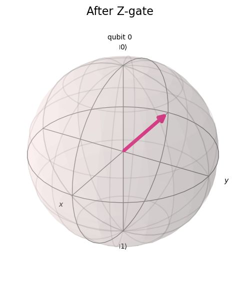
The Z-Gate: Phase Shifter

The Z-gate is a rotation around the Z-axis. Critically, it does not change the probability of measuring '0' or '1' but shifts the internal phase of the |1> angle component.

| Visualization | State Vector (Qiskit Output) | Interpretation | |----|----|----| | Bloch Sphere (After Z-gate): | [0.707 + 0.j, -0.707 + 0.j] | Notice the negative sign on the second amplitude. The measurement probability is still 50/50, but the Z-gate rotated the state vector 180 degrees on the equator (from the positive X-axis to the negative X-axis). This phase shift is vital for quantum interference. |

\ \

\

3. Quantum Entanglement

Quantum entanglement is a phenomenon where two or more quantum particles become linked in such a way that their quantum states are inseparable, regardless of the physical distance between them.

They effectively behave as a single system.

The most famous entangled state is the Bell state, (|00⟩ + |11⟩)/√2, where two qubits are in a superposition of both being 0 and both being 1.

The moment one entangled qubit is measured, the state of the other is instantaneously determined, a feature Einstein called "spooky action at a distance."

This correlation is stronger than any classical correlation and has been experimentally verified through tests of Bell's theorem, disproving classical hidden variable theories.

Entanglement is not just a curiosity; it is a crucial computational resource.

It allows for the creation of complex correlations essential for quantum algorithms like Shor's algorithm, quantum teleportation, and quantum error correction.

Code Example:

This code demonstrates the creation of a four-qubit GHZ (Greenberger–Horne–Zeilinger) state, a form of multi-qubit entanglement where all qubits are perfectly correlated.

\

# Import necessary components from qiskit import QuantumCircuit, transpile from qiskit_aer import AerSimulator from qiskit.visualization import plot_histogram # Create a circuit with 4 qubits and 4 classical bits qc = QuantumCircuit(4, 4) # --- Create the GHZ State --- # 1. Put the first qubit (q0) into superposition qc.h(0) # 2. Cascade CNOT gates to entangle the other qubits with q0 qc.cx(0, 1) qc.cx(0, 2) qc.cx(0, 3) # Add a barrier for visual clarity qc.barrier() # Measure all four qubits qc.measure([0, 1, 2, 3], [0, 1, 2, 3]) # Initialize and run the simulator simulator = AerSimulator() compiled_circuit = transpile(qc, simulator) result = simulator.run(compiled_circuit, shots=1024).result() counts = result.get_counts(qc) # Print the circuit and results print("4-Qubit GHZ State (Multi-Qubit Entanglement) Circuit:") print(qc) print(results)

Output

\ Explanation

This circuit diagram illustrates the creation and measurement of a four-qubit Bell State, also known as an entangled state, where the fate of all four quantum bits are linked.

The circuit links the fate of all four qubits together, a process called entanglement.

The Hadamard (H) gate on the first qubit (q_0) puts it into superposition, meaning it is a 50 percent 0, 50 percent 1 mix.

The subsequent gates are Controlled-NOT (CNOT) gates.

These gates chain the qubits together: if the controlling qubit is 1, the target qubit flips its state.

This cascading structure means the initial superposition of q_0 dictates the state of every other qubit in the chain.

The final state is a superposition of only two possibilities: all four qubits are 0 (0000) or all four are 1 (1111).

The system is guaranteed to be in either one of these states, demonstrating perfect correlation, which is entanglement.

All four qubits are measured and the results are stored.

The output results ('0000': 509, '1111': 515) show that after running the simulation about 1024 times, the result was '0000' half the time and '1111' the other half.

The key takeaway is that you will never see an uncorrelated result like '0101' or '1000' because the qubits are entangled and their values must match.

4. Quantum Gates

Quantum gates are the fundamental building blocks of quantum circuits, analogous to classical logic gates.

They perform operations that manipulate the quantum states of one or more qubits.

A crucial difference is that all quantum operations (except measurement) must be unitary, which implies they are reversible; no information is ever lost.

Key single-qubit gates include the Pauli-X (NOT gate), Pauli-Z (phase-flip gate), and the Hadamard (superposition gate).

The most important two-qubit gate is the Controlled-NOT (CNOT) gate, which flips a target qubit if and only if a control qubit is in the state |1⟩.

The CNOT gate is essential for creating entanglement.

A finite set of gates is considered "universal" if any possible quantum operation can be approximated by a sequence of gates from that set.

Code Example:

This code demonstrates the action of a CNOT gate. It prepares the control qubit in a superposition, allowing the CNOT gate to generate an entangled Bell state.

\

# Import necessary components from qiskit import QuantumCircuit from qiskit.quantum_info import Statevector # Create a circuit with 2 qubits qc = QuantumCircuit(2) # --- Initial State --- # By default, the state is |00> initial_state = Statevector(qc) print("Initial State (|00>):") print(initial_state.draw('text')) # --- Step 1: Create Superposition on Control Qubit --- # Apply a Hadamard gate to the control qubit (q0) qc.h(0) state_after_h = Statevector(qc) print("\nState after H-gate on q0 (Superposition):") print(state_after_h.draw('text')) # --- Step 2: Apply CNOT Gate --- # Apply a CNOT with q0 as control and q1 as target qc.cx(0, 1) final_state = Statevector(qc) print("\nFinal State after CNOT (Entangled Bell State):") print(final_state.draw('text')) print("\nCircuit Diagram:") print(qc)

Output

Explanation

This output shows how to create the simplest entangled state, known as the two-qubit Bell State.

The circuit uses two qubits, q0 and q1. Qubits start in the 00 state.

The first step is applying the Hadamard (H) gate to q_0.

This puts the first qubit into superposition.

The state vector shows the two-qubit system is now split between the 00 state and the 10 state, with equal probability.

The numerical values (0.707…) confirm this 50 percent split. The second qubit (q_1) remains at 0 because it has not been acted on.

The next step is applying the Controlled-NOT (CNOT) gate. The CNOT uses q0 to control q1. The CNOT flips q1 only if q0 is in the 1 state.

The Final State after CNOT is the Entangled Bell State.

The vector shows that the only possibilities left are the 00 state and the 11 state, again with 50 percent probability each.

This perfect correlation is the definition of entanglement.

If you measure the first qubit as 0, the second qubit is guaranteed to be 0.

If you measure the first qubit as 1, the second qubit is guaranteed to be 1.

You will never observe a mixed result like 01 or 10.

\

5. Quantum Circuits

A quantum circuit is the standard model for quantum computation, providing a visual framework for how an algorithm is executed.

It depicts the flow of qubits over time, from left to right, as they undergo a sequence of quantum gate operations.

Horizontal lines represent the qubits, while boxes on these lines represent the applied quantum gates.

The circuit begins with qubits initialized in a specific state, typically all |0⟩.

The gates then manipulate these states, creating superposition and entanglement to perform the computation.

The circuit concludes with measurement operations, which extract classical information (0s and 1s) from the final quantum state.

A circuit's complexity is defined by its width (number of qubits) and depth (longest path of sequential gates).

Circuit depth is a critical metric for today's noisy quantum devices, as shallower circuits are less susceptible to errors from decoherence.

Code Example:

This code builds a quantum half-adder that adds two bits (1 + 1). The inputs are encoded on q0 and q1, with the sum measured from q1 and the carry from q2.

\

# Import necessary components from qiskit import QuantumCircuit, transpile from qiskit_aer import AerSimulator # Create a circuit with 3 qubits and 2 classical bits # q0: input A # q1: input B / output Sum # q2: output Carry qc = QuantumCircuit(3, 2) # --- Prepare Inputs --- # We want to compute 1 + 1, so we set q0 and q1 to |1> qc.x(0) qc.x(1) qc.barrier() # --- Half-Adder Logic --- # 1. Calculate the Carry bit (A AND B) # The Toffoli gate (ccx) flips the target (q2) if both controls (q0, q1) are 1. qc.ccx(0, 1, 2) # 2. Calculate the Sum bit (A XOR B) # The CNOT gate flips the target (q1) if the control (q0) is 1. qc.cx(0, 1) qc.barrier() # --- Measurement --- # Measure the Sum (q1) and Carry (q2) qc.measure(1, 0) # Map q1 to classical bit 0 (Sum) qc.measure(2, 1) # Map q2 to classical bit 1 (Carry) # Simulate the circuit simulator = AerSimulator() compiled_circuit = transpile(qc, simulator) result = simulator.run(compiled_circuit, shots=1).result() counts = result.get_counts() # Print the circuit and the result print("Quantum Half-Adder Circuit for 1 + 1:") print(qc)

Output

Explanation

This circuit is a Quantum Half-Adder performing the binary sum 1 + 1.

• Input Setup: The X gates set the two input qubits ($q0, q1$) to the value 1.
• Carry Calculation: The three-part gate (two dots and an X on q2) calculates the Carry (the AND operation).
• Since the input is 1+1, the carry qubit (q2) flips to 1.
• Sum Calculation: The remaining gates calculate the Sum (the XOR operation), which results in 0 for 1+1.
• Output: The final measurement reads the carry (1) and the sum (0), giving the binary result 10, which equals the number two.

\

6. Quantum Simulators

A quantum simulator is a classical (traditional) computer program designed to mimic the behavior of a real quantum computer.

Since building and operating large, stable quantum hardware is immensely difficult, simulators are the primary tool used by developers and researchers to test algorithms and circuits.

Quantum simulators work by representing the quantum state of a circuit—the amplitudes and probabilities of all possible outcomes—as a large, complex vector stored in the classical computer's memory.

When a quantum gate is applied, the simulator performs a complex matrix multiplication on this vector, accurately predicting how a real quantum computer would behave.

The core limitation of quantum simulators is memory.

For every additional qubit, the required memory (RAM) doubles exponentially (2^N) where N is the number of qubits).

While a classical computer can easily simulate a 20-qubit circuit (requiring about 1 GB of RAM), simulating 50 qubits is practically impossible, as it would require petabytes of memory—this boundary is known as quantum supremacy or the point where quantum hardware outperforms classical simulation.

Code Example:

This code demonstrates using Qiskit's built-in state vector simulator (Aer) to execute a quantum circuit and inspect the final probability distribution of the outcomes.

# Import necessary components from qiskit import QuantumCircuit from qiskit_aer import Aer from qiskit.visualization import plot_histogram # Create a circuit with one qubit qc = QuantumCircuit(1) # Apply a Hadamard gate to create superposition (50/50 chance) qc.h(0) # Measure the final state qc.measure_all() # --- Run the simulation 1024 times --- # Use the Qiskit Aer simulator backend simulator = Aer.get_backend('qasm_simulator') job = simulator.run(qc, shots=1024) result = job.result() counts = result.get_counts(qc) print("Circuit:") print(qc) # Plotting the histogram shows the simulated probabilities plot_histogram(counts, title="Simulation Results (50/50)").savefig("Q6.png")

Output

Explanation

The qubit starts at 0.

The Hadamard (H) gate creates superposition, setting the probability of measuring 0 or 1 to 50 percent each.

The subsequent measurement forces a choice.

Running the experiment 1024 times confirms this randomness, resulting in a near 50/50 split (507 results for 0, 517 for 1).

7. Quantum Measurement

Quantum measurement is the process of extracting classical information from a quantum system.

It is a fundamentally probabilistic and irreversible operation.

Unlike in classical physics, the act of measurement actively alters the quantum system, causing the collapse of the state vector.

When a qubit in superposition α|0⟩ + β|1⟩ is measured, it is forced to choose one of the basis states.

The qubit will collapse to |0⟩ with a probability of |α|² and to |1⟩ with a probability of |β|².

Once measured, the qubit's superposition is destroyed, and it now holds a definite classical value.

Quantum algorithms are designed to manipulate the final quantum state so that the desired answer has the highest probability of being measured.

A computation is typically run for many "shots" to build up statistics and infer the most probable, correct answer.

Code Example

This code prepares a qubit in a biased superposition, where the probability of measuring '1' is engineered to be 75%. The measurement statistics from 4096 shots will reflect this bias.

\

# Import necessary components import numpy as np from qiskit import QuantumCircuit, transpile from qiskit_aer import AerSimulator from qiskit.visualization import plot_histogram # Create a circuit with one qubit and one classical bit qc = QuantumCircuit(1, 1) # --- Prepare a Biased Superposition --- # A Y-rotation by angle theta sets the state to cos(theta/2)|0> + sin(theta/2)|1>. # To get Prob(1) = 0.75, we need sin(theta/2) = sqrt(0.75), so theta = 2 * arcsin(sqrt(0.75)) = pi * 2/3. angle = 2 * np.pi / 3 qc.ry(angle, 0) # --- Measurement --- qc.measure(0, 0) # Simulate the circuit shots = 4096 simulator = AerSimulator() compiled_circuit = transpile(qc, simulator) result = simulator.run(compiled_circuit, shots=shots).result() counts = result.get_counts(qc) # Print the results and theoretical probabilities print("Circuit with Biased Superposition (75% |1>):") print(qc) print(counts)

Output

Explanation

This circuit creates a biased superposition.

The Ry gate acts like a dimmer switch, setting the probability of measuring 1 to 75% and 0 to 25%.

The results confirm this bias: after 4096 runs, the outcome 1 was recorded 3002 times, clearly showing the three-to-one probability advantage. .

8. No-Cloning Theorem

The no-cloning theorem is a fundamental principle stating that it is impossible to create an identical, independent copy of an arbitrary, unknown quantum state.

This is not a technological limitation but a direct consequence of the linearity of quantum mechanics.

The theorem distinguishes quantum information from classical information, which can be copied perfectly.

This principle is the bedrock of quantum cryptography and protocols like Quantum Key Distribution (QKD).

It guarantees that an eavesdropper cannot intercept and copy a quantum transmission without disturbing the original state, thus revealing their presence.

The theorem applies only to unknown states; if one knows the exact description of a state, one can prepare another system in that same state, but this is preparation, not cloning.

Code Example

This code demonstrates the no-cloning theorem by comparing a hypothetical "perfectly cloned" state with the actual state produced by a physical copy operation (a CNOT gate). The difference proves that a perfect clone is not created.

\

# Import necessary components import numpy as np from qiskit import QuantumCircuit from qiskit.quantum_info import Statevector # --- Define an arbitrary initial state for one qubit --- # This is the state we want to clone. initial_state_vector = np.array([np.sqrt(0.7), np.sqrt(0.3)]) # --- Calculate the "perfect" cloned state vector (hypothetical) --- # A perfect clone would be the tensor product of the state with itself. perfect_clone_state = np.kron(initial_state_vector, initial_state_vector) # --- Build a circuit that attempts to "clone" the state --- # We initialize q0 to our arbitrary state and try to copy it to q1. qc = QuantumCircuit(2) qc.initialize(initial_state_vector, 0) # Prepare q0 in the desired state qc.cx(0, 1) # Use a CNOT as a "copying" mechanism # --- Get the actual final state vector from the circuit --- actual_final_state = Statevector(qc) # --- Compare the states --- print("Initial State to Clone: |psi> = sqrt(0.7)|0> + sqrt(0.3)|1>") print("\nHypothetical 'Perfect' Cloned State |psi>|psi>:") print(np.round(perfect_clone_state, 3)) print("\nActual State from CNOT 'Copy' Circuit:") print(np.round(actual_final_state.data, 3))

Output

Explanation:

The goal of this process is to take an initial unknown state (psi) and copy it onto a second qubit, resulting in the desired state (psi)(psi).

\

• Initial State to Clone: The qubit starts in a specific superposition: psi equals square root of 0.7 times the 0 state plus square root of 0.3 times the 1 state. This means the qubit has a 70 percent chance of being measured as 0 and a 30 percent chance of being measured as 1.

\

• Hypothetical Perfect Clone: If cloning were possible, the resulting two-qubit vector would look like the Hypothetical Perfect Cloned State vector. This vector represents two perfectly identical, independent copies of the initial state.

\

• The Failed Attempt (CNOT Copy Circuit): A simple CNOT gate is often used in an attempt to copy the state. However, the Actual State from CNOT Copy Circuit vector clearly shows that the CNOT operation failed to create the perfect copy.

  \

• Analysis: The final vector does not match the Hypothetical Vector. Instead of two independent copies, the CNOT operation created an entangled state. The final non-zero amplitudes correspond only to the 00 state and the 11 state, which demonstrates entanglement rather than two separate, identical qubits.

This outcome confirms the No Cloning Theorem: you cannot create a perfect duplicate of an unknown quantum state.

This principle is vital for the security of quantum communication.

\

9. Quantum Teleportation

Quantum teleportation is a protocol that transfers a quantum state from one location to another without physically moving the particle carrying the state.

The protocol relies on two key quantum resources: entanglement and classical communication.

It requires three qubits: a source qubit |ψ⟩ (held by "Alice") and a pre-shared entangled pair, with one half held by Alice and the other by the receiver, "Bob".

1. Alice performs a joint Bell measurement on her source qubit and her half of the entangled pair.
2. She sends the two classical bits from her measurement to Bob over a classical channel.
3. Bob then applies one of four specific correction gates to his qubit, determined by the bits he received.
4. After the correction, Bob's qubit is transformed into an exact replica of Alice's original state |ψ⟩, which was destroyed in the process, upholding the no-cloning theorem.

Code Example

This code provides a full implementation of the quantum teleportation protocol, teleporting an arbitrary state from qubit q0 to qubit q2.

\

# Import necessary components import numpy as np from qiskit import QuantumCircuit from qiskit.quantum_info import Statevector # --- Step 0: Create an arbitrary state to teleport --- source_qc = QuantumCircuit(1) initial_angle = np.pi / 3 # An arbitrary angle source_qc.ry(initial_angle, 0) initial_state = Statevector(source_qc) # --- The Main Teleportation Circuit (with measurements and control flow) --- qc = QuantumCircuit(3, 2) # Step 1: Initialize Alice's source qubit qc.ry(initial_angle, 0) qc.barrier() # Step 2: Create an entangled Bell pair between q1 and q2 qc.h(1) qc.cx(1, 2) qc.barrier() # Step 3: Alice performs a Bell measurement qc.cx(0, 1) qc.h(0) qc.barrier() # Step 4: Alice measures her qubits and sends classical bits qc.measure(0, 0) qc.measure(1, 1) qc.barrier() # Step 5: Bob applies corrections based on classical bits with qc.if_test((qc.clbits[1], 1)): qc.x(2) with qc.if_test((qc.clbits[0], 1)): qc.z(2) # --- Verification: Show teleportation works for all outcomes --- print("=" * 60) print("QUANTUM TELEPORTATION DEMONSTRATION") print("=" * 60) print("\nQuantum Teleportation Circuit:") print(qc) print("\n" + "=" * 60) print("INITIAL STATE (Alice's qubit q0):") print("=" * 60) print(initial_state.draw('text')) print("\n" + "=" * 60) print("FINAL STATE (Bob's qubit q2) for each measurement outcome:") print("=" * 60) # Check all four possible measurement outcomes for m0 in [0, 1]: for m1 in [0, 1]: # Build circuit for this specific outcome outcome_qc = QuantumCircuit(1) outcome_qc.ry(initial_angle, 0) # Simulate the teleportation with corrections for this outcome # The Bell measurement projects the state, then Bob applies corrections # After corrections, q2 should have the original state # For outcome |m0,m1>, Bob applies: # X gate if m1 = 1 # Z gate if m0 = 1 if m1 == 1: outcome_qc.x(0) if m0 == 1: outcome_qc.z(0) final_state = Statevector(outcome_qc) print(f"\nMeasurement outcome |{m0}{m1}>:") print(f" Bob applies: ", end="") corrections = [] if m1 == 1: corrections.append("X") if m0 == 1: corrections.append("Z") print(", ".join(corrections) if corrections else "No corrections") print(f" Bob's final state:") print(final_state.draw('text')) print("\n" + "=" * 60) print("VERIFICATION:") print("=" * 60) print("Initial state on q0:") print(initial_state) print("\nBob's state after teleportation (any outcome):") print(Statevector(source_qc)) print("\n✓ Teleportation successful! Bob's qubit matches Alice's original state.")

Output

Explanation

This verifies the Quantum Teleportation protocol.

The Protocol's Goal

The goal of Quantum Teleportation is to transfer the state of an unknown qubit (Alice's initial state) to a different qubit held by Bob, using a pre-shared entangled pair and classical communication.

Crucially, the process destroys the state on Alice's side but recreates it perfectly on Bob's side, without physically transporting the qubit.

Step-by-Step State Corrections

Alice performs a measurement on her two qubits (the unknown state and her half of the entangled pair).

The four possible two-bit outcomes (00, 01, 10, 11) tell Bob exactly which correctional gate(s) he must apply to his entangled qubit to complete the teleportation.

| Measurement Outcome | Alice's Observation | Bob Applies | Bob's Final State | |----|----|----|----| | 00 | No effect on his qubit. | No corrections | State matches initial state. | | 01 | His qubit requires a flip. | X (NOT) gate | State matches initial state. | | 10 | His qubit requires a phase shift. | Z (Phase) gate | State matches initial state. | | 11 | His qubit requires a flip and a phase shift. | X and Z gates | State matches initial state. |

\ Verification

The verification section confirms that, regardless of which of the four outcomes occurred, Bob successfully recreated the state.

• Initial state on q0: This is the original, unknown state Alice wanted to send (e.g., $0.866…|0\rangle + 0.5|1\rangle$).
• Bob's state after teleportation (any outcome): This shows that after applying the necessary correction(s), Bob's qubit state vector is identical to Alice's initial state vector.
• Which means that the teleportation is successful.

\

10. Decoherence

Decoherence is the single greatest obstacle to building large-scale, fault-tolerant quantum computers.

It is the process by which a quantum system loses its quantum properties—superposition and entanglement—through interaction with its environment.

These interactions effectively "leak" information about the qubit's state, which is equivalent to the environment "measuring" the qubit.

This unintended measurement forces the quantum state to collapse, destroying its coherence and corrupting the computation.

Decoherence manifests in two primary ways: Energy Relaxation (T1 time), where a qubit decays to its ground state, and Dephasing (T2 time), where the relative phase of a superposition is randomized.

The goal of quantum hardware engineers is to maximize these coherence times while minimizing gate operation times.

Strategies to combat decoherence include extreme isolation (cryogenic temperatures), designing more robust qubits, and implementing quantum error correction.

Prerequisites: qiskit, qiskit-aer

Code Example:

This code simulates a Ramsey experiment to show the effect of T2 dephasing. An ideal qubit returns to |0⟩, while a noisy qubit will show an increased probability of being measured as |1⟩ due to loss of phase coherence.

\

# Import necessary components from qiskit import QuantumCircuit, transpile from qiskit_aer import AerSimulator from qiskit_aer.noise import NoiseModel, phase_amplitude_damping_error from qiskit.visualization import plot_histogram # --- Simulation Parameters --- delay_time = 100 # Arbitrary time unit for the delay # --- Ideal Simulation (No Noise) --- ideal_qc = QuantumCircuit(1, 1) ideal_qc.h(0) ideal_qc.delay(delay_time, 0, unit='ns') # Wait for some time ideal_qc.h(0) ideal_qc.measure(0, 0) ideal_sim = AerSimulator() ideal_result = ideal_sim.run(transpile(ideal_qc, ideal_sim), shots=1024).result() ideal_counts = ideal_result.get_counts() # --- Noisy Simulation (With Decoherence) --- # Create a noise model with T1=1000ns and T2=500ns. t1_time = 1000 t2_time = 500 decoherence_error = phase_amplitude_damping_error( t1_time, t2_time, excited_state_population=0 ) noise_model = NoiseModel() noise_model.add_all_qubit_quantum_error(decoherence_error, ['delay']) noisy_sim = AerSimulator(noise_model=noise_model) noisy_result = noisy_sim.run(transpile(ideal_qc, noisy_sim), shots=1024).result() noisy_counts = noisy_result.get_counts() # --- Print Results --- print("Ramsey Experiment Simulation") print("\nIdeal Results (No Decoherence):") print(ideal_counts) print("\nNoisy Results (With T2 Dephasing):") print(noisy_counts)

Output:

Explanation:

\

1. The image displays a Ramsey-style quantum circuit experiment executed under two conditions: ideal (noiseless) and noisy.
2. The circuit applies a Hadamard gate, waits for a 100 nanosecond delay, applies a second Hadamard gate, and then measures the result.
3. In an ideal quantum system, two consecutive Hadamard gates cancel each other out, which should return the qubit to its initial state of 0.
4. The Ideal Results confirm this theory, showing that all 1024 simulation shots resulted in a measurement of 0.
5. The second circuit represents a realistic scenario where the qubit is subject to environmental noise during the 100 nanosecond idle delay.
6. The Noisy Results show that the state is no longer pure, with 103 shots resulting in a 1 and 921 shots resulting in a 0.
7. This shift happens because T1 thermal relaxation and T2 dephasing errors cause the qubit to lose its quantum information while it is waiting.
8. This comparison illustrates how decoherence limits the amount of time a qubit can maintain a superposition state before errors occur.

Epilogue: The Future of Quantum Computing in 2025

The year 2025 stands as a pivotal moment in the quantum timeline, marking a transition from an era of academic curiosity and noisy, small-scale devices toward a new phase of engineering-driven progress and the quest for practical quantum advantage.

The primary focus is the relentless scaling of quantum hardware, with leading platforms expected to feature processors containing several hundred to over a thousand physical qubits, a significant leap from the sub-hundred-qubit devices of the early 2020s.

This increase in qubit count is coupled with an even more critical push for quality over quantity, with major efforts dedicated to improving two-qubit gate fidelities to well beyond 99.9% and extending qubit coherence times, which are essential for running deeper, more meaningful quantum circuits.

Quantum error correction is moving from theoretical frameworks to experimental reality, with 2025 seeing the first demonstrations of logical qubits that are actively stabilized and possess lifetimes significantly longer than their individual physical constituent qubits, a landmark achievement on the road to fault tolerance.

Hybrid quantum-classical algorithms remain the dominant paradigm for near-term applications, with more sophisticated variational methods and quantum machine learning models being developed to maximize the utility of noisy intermediate-scale quantum (NISQ) hardware.

The field of quantum chemistry simulation is poised to achieve practical advantage, with quantum computers in 2025 being used to model molecules of industrial relevance, such as catalysts or pharmaceutical compounds, with an accuracy that begins to challenge the best classical supercomputers.

In finance, quantum algorithms for optimization and risk analysis are being deployed on a larger scale, moving from proof-of-concept experiments to integrated workflows that tackle real-world portfolio optimization and derivative pricing problems.

The software stack for quantum computing is maturing rapidly, with higher-level programming languages and sophisticated compiler optimizations that abstract away the complexities of the underlying hardware, making quantum development more accessible to domain experts who are not quantum physicists.

Cloud access to quantum computers is becoming ubiquitous, with multiple hardware providers offering their systems through integrated platforms, fostering a growing ecosystem of software startups and enterprise research teams dedicated to building quantum-ready applications.

Despite this progress, the dream of a universal, fault-tolerant quantum computer capable of running algorithms like Shor's to break modern encryption remains a more distant goal, with the challenges of large-scale error correction and system integration defining the next frontier of quantum engineering.

\

\

References

1. Nielsen, M. A., & Chuang, I. L. (2010). Quantum Computation and Quantum Information: 10th Anniversary Edition. Cambridge University Press. (The foundational textbook of the field).
2. Qiskit Textbook. IBM. An open-source online textbook that provides an interactive introduction to quantum computing. https://qiskit.org/textbook/content/ch-ex/
3. Preskill, J. (1998). Lecture Notes for Physics 229: Quantum Information and Computation. California Institute of Technology. http://www.theory.caltech.edu/~preskill/ph229/
4. Arute, F., Arya, K., Babbush, R. et al. (2019). Quantum supremacy using a programmable superconducting processor. Nature 574, 505–510. https://www.nature.com/articles/s41586-019-1666-5
5. Quanta Magazine. An editorially independent online publication of the Simons Foundation that provides in-depth coverage of quantum computing developments. https://www.quantamagazine.org/tag/quantum-computing/
6. arXiv Quantum Physics Archive. A repository for pre-print academic papers, where most new research in the field is published. https://arxiv.org/archive/quant-ph

\

:::tip Stay tuned for Part II - 10 Not So Easy Pieces!

:::

\

:::info All images were AI-generated by the author with NightCafe Studio, available here: https://creator.nightcafe.studio/explore

:::

\

:::info Google AI Studio was used in this article, available here: https://aistudio.google.com/

:::

\ \ \ \