

How PDE Motion Models Boost Image Reconstruction in Dynamic CT
:::info Authors:
(1) Pablo Arratia, University of Bath, Bath, UK (pial20@bath.ac.uk);
(2) Matthias Ehrhardt, University of Bath, Bath, UK (me549@bath.ac.uk);
(3) Lisa Kreusser, University of Bath, Bath, UK (lmk54@bath.ac.uk).
:::
Table of Links
Abstract and 1. Introduction
-
Dynamic Inverse Problems in Imaging
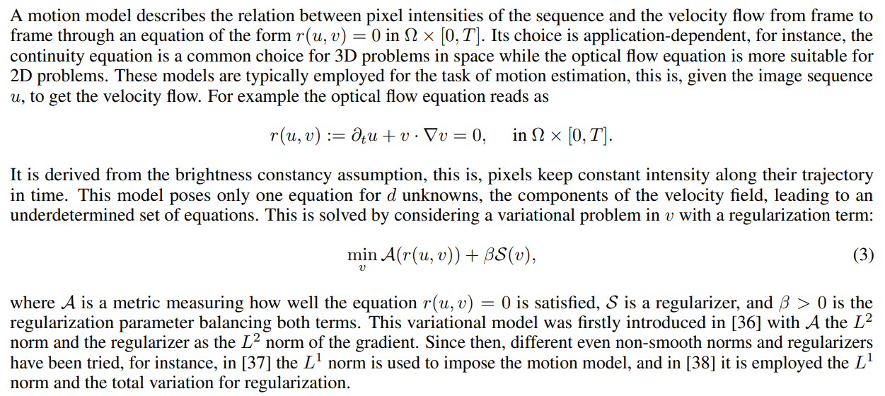
2.1 Motion Model
2.2 Joint Image Reconstruction and Motion Estimation
-
Methods
3.1 Numerical evaluation with Neural Fields
3.2 Numerical evaluation with grid-based representation
-
Numerical Experiments
4.1 Synthetic experiments
-
Conclusion, Acknowledgments, and References
ABSTRACT
Image reconstruction for dynamic inverse problems with highly undersampled data poses a major challenge: not accounting for the dynamics of the process leads to a non-realistic motion with no time regularity. Variational approaches that penalize time derivatives or introduce PDE-based motion model regularizers have been proposed to relate subsequent frames and improve image quality using grid-based discretization. Neural fields are an alternative to parametrize the desired spatiotemporal quantity with a deep neural network, a lightweight, continuous, and biased towards smoothness representation. The inductive bias has been exploited to enforce time regularity for dynamic inverse problems resulting in neural fields optimized by minimizing a data-fidelity term only. In this paper we investigate and show the benefits of introducing explicit PDE-based motion regularizers, namely, the optical flow equation, in 2D+time computed tomography for the optimization of neural fields. We also compare neural fields against a grid-based solver and show that the former outperforms the latter.
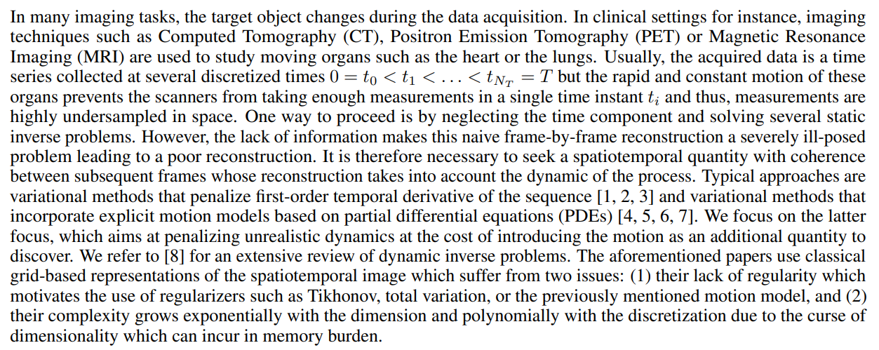
1 Introduction
\ 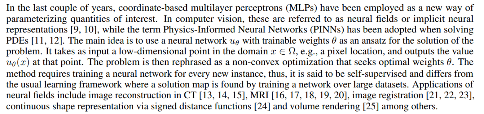
\ It is well-known that, under mild conditions, neural networks can approximate functions at any desired tolerance [26], but their widespread use has been justified by other properties such as (1) the implicit regularization they introduce, (2) overcoming the curse of dimensionality, and (3) their lightweight, continuous and differentiable representation. In [27, 28] it is shown that the amount of weights needed to approximate the solution of particular PDEs grows polynomially on the dimension of the domain. For the same reason, only a few weights can represent complex images, leading to a compact and memory-efficient representation. Finally, numerical experiments and theoretical results show that neural fields tend to learn smooth functions early during training [29, 30, 31]. This is both advantageous and disadvantageous: neural fields can capture smooth regions of natural images but will struggle at capturing edges. The latter can be overcome with Fourier feature encoding [32].
\ In the context of dynamic inverse problems and neural fields, most of the literature relies entirely on the smoothness introduced by the network on the spatial and temporal variables to get a regularized solution. This allows minimizing a data-fidelity term only without considering any explicit regularizers. Applications can be found on dynamic cardiac MRI in [17, 20, 19], where the network outputs the real and imaginary parts of the signal, while in [18] the neural field is used to directly fit the measurements and then inference is performed by inpainting the k-space with the neural field and taking the inverse Fourier transform. In [33, 34] neural fields are used to solve a photoacoustic tomography dynamic reconstruction emphasizing their memory efficiency. In [15], a 3D+time CT inverse problem is addressed with a neural field parametrizing the initial frame and a polynomial tensor warping it to get the subsequent frames. To the best of our knowledge, it is the only work making use of neural fields and a motion model via a deformable template.
\ In this paper, we investigate the performance of neural fields regularized by explicit PDE-based motion models in the context of dynamic inverse problems in CT in a highly undersampled measurement regime with two dimensions in space. Motivated by [4] and leveraging automatic differentiation to compute spatial and time derivatives, we study the optical flow equation as an explicit motion regularizer imposed as a soft constraint as in PINNs. Our findings are based on numerical experiments and are summarized as follows:
\ • An explicit motion model constraints the neural field into a physically feasible manifold improving the reconstruction when compared to a motionless model.
\ • Neural fields outperform grid-based representations in the context of dynamic inverse problems in terms of the quality of the reconstruction.
\ • We show that, once the neural field has been trained, it generalizes well into higher resolutions.
\ The paper is organized as follows: in section 2 we introduce dynamic inverse problems, motion models and the optical flow equation, and the joint image reconstruction and motion estimation variational problem as in [4]; in section 3 we state the main variational problem to be minimized and study how to minimize it with neural fields and with a grid-based representation; in section 4 we study our method on a synthetic phantom which, by construction, perfectly satisfies the optical flow constraint, and show the improvements given by explicit motion regularizers; we finish with the conclusions in section 5.
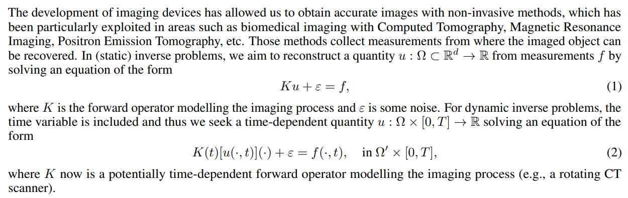
2 Dynamic Inverse Problems in Imaging
2.1 Motion Model
\
2.2 Joint Image Reconstruction and Motion Estimation
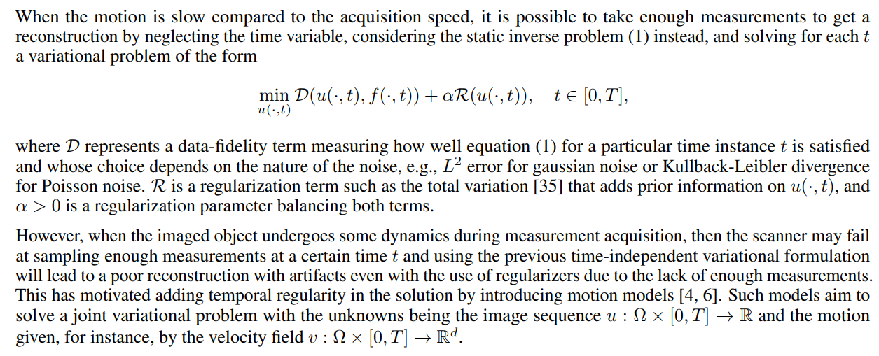
To solve highly-undersampled dynamic inverse problems, in [4] it is proposed a joint variational problem where not only the dynamic process u is sought, but also the underlying motion expressed in terms of a velocity field v. The main hypothesis is that a joint reconstruction can enhance the discovery of both quantities, image sequence and motion, improving the final reconstruction compared to motionless models. Hence, the sought solution (u ∗ , v∗ ) is a minimizer for the variational problem given below:
\ 
\ with α, β, γ > 0 being regularization parameters balancing the four terms. In [4], the domain is 2D+time, and among others, it is shown how the purely motion estimation task of a noisy sequence can be enhanced by solving the joint task of image denoising and motion estimation.
\ This model was further employed for 2D+time problems in [6] and [7]. In the former it is studied its application on dynamic CT with sparse limited-angles and it is studied both L 1 and L 2 norms for the data fidelity term, with better results for the former. In the latter, the same logic is used for dynamic cardiac MRI. In 3D+time domains, we mention [39] and [40] for dynamic CT and dynamic photoacoustic tomography respectively.
\
3 Methods
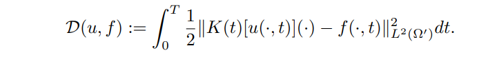
Depending on the nature of the noise, different data-fidelity terms can be considered. In this work, we consider Gaussian noise ε, so, to satisfy equation (2) we use an L2 distance between predicted measurements and data
\ 
\ Since u represents a natural image, a suitable choice for regularizer R is the total variation to promote noiseless images and capture edges:
\ 
\ For the motion model, we consider the optical flow equation (5), and to measure its distance to 0 we use the L1 norm. For the regularizer in v we consider the total variation on each of its components.
\ 
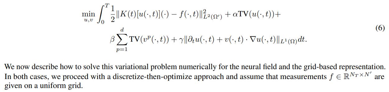
\ Thus, the whole variational problem reads as follows:
\ 
\
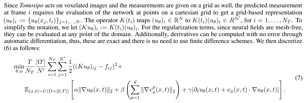
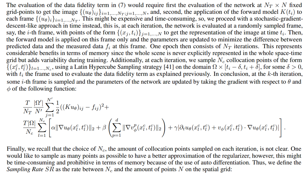
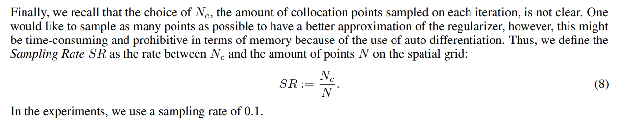
3.1 Numerical evaluation with Neural Fields
\ 
\ 
\
3.2 Numerical evaluation with grid-based representation
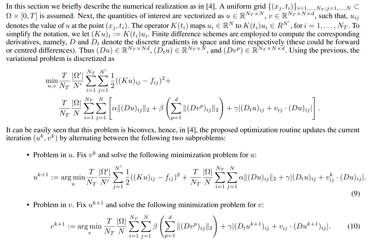
\ Each subproblem is convex with non-smooth terms involved that can be solved using the Primal-Dual Hybrid Gradient (PDHG) algorithm [42]. We refer to [4] for the details.
\
:::info This paper is available on arxiv under CC BY 4.0 DEED license.
:::
\
You May Also Like

Buterin pushes Layer 2 interoperability as cornerstone of Ethereum’s future

Trump family-affiliated company Thumzup invests $2.5 million in DogeHash Technologies
